How to compare data in Excell by using Vlookup and Match Functions

In this article I am going to explain how to compare two excel
sheets data and highlight the missing data. This article is helpful in BPO
industry those who are dealt with finance and insurance sector.

Now a day’s everything automated in this comparison of two excel
sheets is taking too lengthy process and our eyes also gets strained so to
avoid that read the article and practice yourself with a sample data. If you
have any questions let me know.

Here I am using two functions 

VLOOKUP()

       MATCH()

Usage of VLOOKUP() function in excel:

Syntax of Vlookup function: 

First go to formulas tab and select Lookup & Reference
then click on VLOOKUP():

 Based on the syntax of the function pass the values like below:

Lookup Value - > What is the required value for searching.

Table Array -> Select the range where you want to find the given element.

Column Index -> Column number 

Range Lookup -> True or False

See the below practice excel sheet which contains the data:

 

By Using MATCH() Function:

Match Function Syntax:

 

 Go to formulas tab and select Lookup & Reference
then click on MATCH().

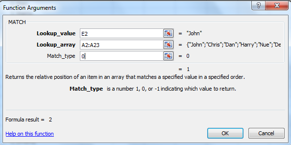
Fill the formula columns like below:

Look up value -> What the element you want to search, select that column.

Look up array -> Where you want to search the element select the range.

Match Type -> It is 0,1,-1  0 for exact match 1 or -1 greater than or less than

See the below practice excel sheet which contains the data:

 

PLEASE NOTE : in the above practice sheet NA means no match found.